Installing package into 'C:/Users/Rebecca/AppData/Local/R/win-library/4.3'
(as 'lib' is unspecified)
Warning: package 'Smarket' is not available for this version of R

A version of this package for your version of R might be available elsewhere,
see the ideas at
https://cran.r-project.org/doc/manuals/r-patched/R-admin.html#Installing-packages
Warning: unable to access index for repository http://www.stats.ox.ac.uk/pub/RWin/bin/windows/contrib/4.3:
  cannot open URL 'http://www.stats.ox.ac.uk/pub/RWin/bin/windows/contrib/4.3/PACKAGES'
Warning in p_install(package, character.only = TRUE, ...):
Warning in library(package, lib.loc = lib.loc, character.only = TRUE,
logical.return = TRUE, : there is no package called 'Smarket'
Warning in p_load("ISLR", "MASS", "descr", "Smarket", "leaps", "tidyverse", : Failed to install/load:
Smarket
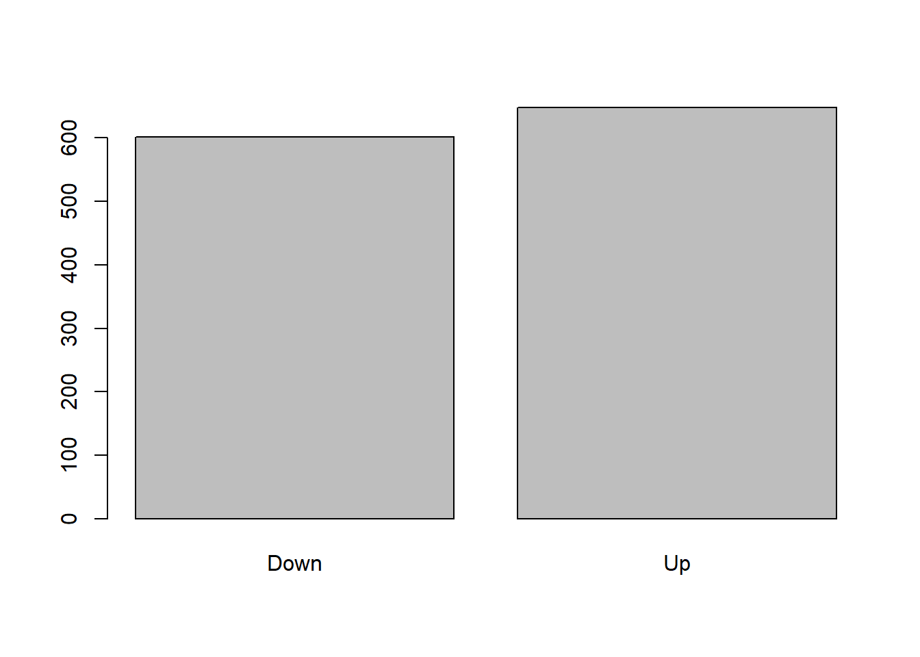
## Make sure libraries are loading. Had some trouble with this. require(ISLR)require(MASS)require(descr)attach(Smarket)## Linear Discriminant Analysisfreq(Direction)
Direction
      Frequency Percent
Down        602   48.16
Up          648   51.84
Total      1250  100.00
Call:
lda(Direction ~ Lag1 + Lag2, data = Smarket, subset = Year <
    2005)

Prior probabilities of groups:
    Down       Up
0.491984 0.508016

Group means:
            Lag1        Lag2
Down  0.04279022  0.03389409
Up   -0.03954635 -0.03132544

Coefficients of linear discriminants:
            LD1
Lag1 -0.6420190
Lag2 -0.5135293
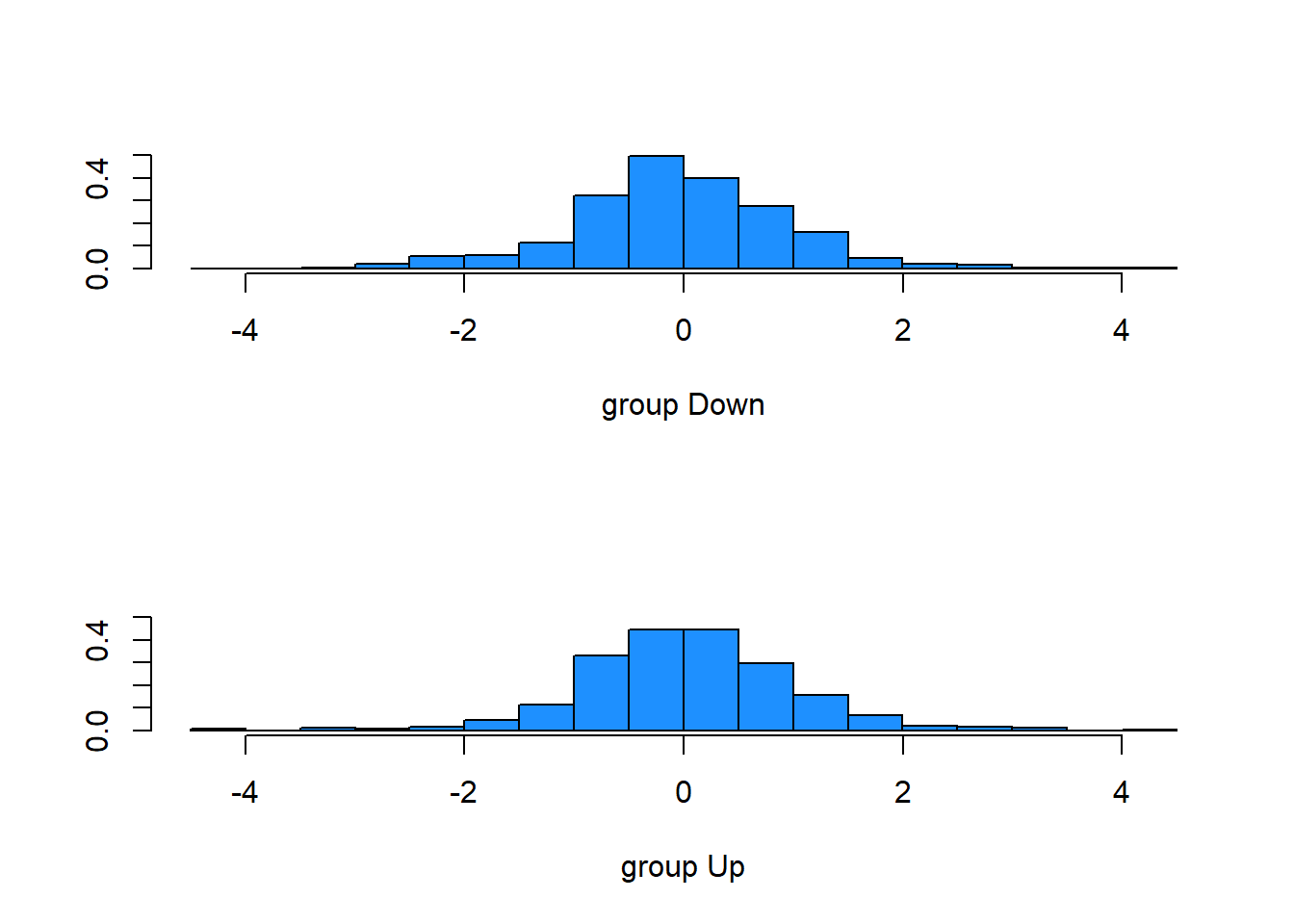
plot(lda.fit, col="dodgerblue")
Smarket.2005=subset(Smarket,Year==2005) # Creating subset with 2005 data for predictionlda.pred=predict(lda.fit,Smarket.2005)names(lda.pred)
         Direction.2005
lda.class Down  Up
     Down   35  35
     Up     76 106
data.frame(lda.pred)[1:5,]
     class posterior.Down posterior.Up         LD1
999     Up      0.4901792    0.5098208  0.08293096
1000    Up      0.4792185    0.5207815  0.59114102
1001    Up      0.4668185    0.5331815  1.16723063
1002    Up      0.4740011    0.5259989  0.83335022
1003    Up      0.4927877    0.5072123 -0.03792892
table(lda.pred$class,Smarket.2005$Direction)
       Down  Up
  Down   35  35
  Up     76 106
mean(lda.pred$class==Smarket.2005$Direction)
[1] 0.5595238
Assignment Questions
From the three methods (best subset, forward stepwise, and backward stepwise):
Which of the three models with k predictors has the smallest training RSS?
Best subset selection has the smallest training RSS. Forward stepwise and backward stepwise have path dependence which can result in an early bad selection impacting the quality of the model overall.
Which of the three models with k predictors has the smallest test RSS?
It depends, because it is possible that all approaches end up with the same model or the forward and backward stepwise select a better model. Generally speaking, again best subset has the smallest test RSS because it considers every model given the input predictors.
Application Exercise
#Generate simulated data set.seed(1)X <-rnorm(100)eps <-rnorm(100)
#Generate a response vector y of length n = 100 according to the modelY <-3+1*X +4*X^2-1*X^3+ eps
#Use the leaps package
library(leaps)
#Use regsubsets() function to perform best subset selectionfit1 <-regsubsets(Y~poly(X,10,raw=T), data=data.frame(Y,X), nvmax=10)summary1 <-summary(fit1)
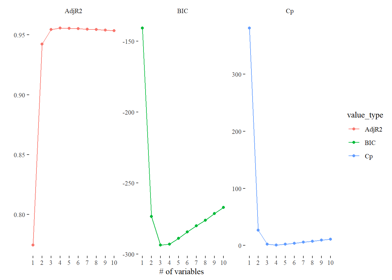
#What is the best model according to Cp, BIC, and adjust R^2? Show plots and report coefficients. data_frame(Cp = summary1$cp,BIC = summary1$bic,AdjR2 = summary1$adjr2) %>%mutate(id =row_number()) %>%gather(value_type, value, -id) %>%ggplot(aes(id, value, col = value_type)) +geom_line() +geom_point() +ylab('') +xlab('# of variables') +facet_wrap(~ value_type, scales ='free') +theme_tufte() +scale_x_continuous(breaks =1:10)
Warning: `data_frame()` was deprecated in tibble 1.1.0.
ℹ Please use `tibble()` instead.
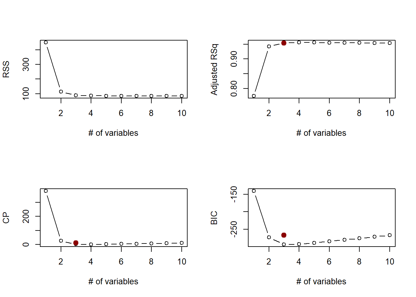
par(mfrow =c(2,2))plot(summary1$rss, xlab ="# of variables", ylab ="RSS", type ="b")which.min(summary1$rss)
[1] 10
points(11, summary1$rss[10], col ="darkred", cex =2, pch =20)plot(summary1$adjr2, xlab ="# of variables",ylab ="Adjusted RSq", type ="b")which.max(summary1$adjr2)
[1] 4
points(3, summary1$adjr2[10], col ="darkred", cex =2, pch =20)plot(summary1$cp, xlab ="# of variables", ylab ="CP", type ="b")which.min(summary1$cp)
[1] 4
points(3, summary1$cp[10], col ="darkred", cex =2, pch =20)plot(summary1$bic, xlab ="# of variables", ylab ="BIC", type ="b")which.min(summary1$bic)
[1] 3
points(3, summary1$bic[10], col ="darkred", cex =2, pch =20)
3 is the optimal number of variables to include as predictors.