Assignment 7

Author

Rebecca Larsen

Run lab logisticregression01 by Dr. Karl Ho

# Load ISLR library

require(ISLR)

Loading required package: ISLR

Warning: package 'ISLR' was built under R version 4.2.3

# Check dataset Smarket
?Smarket

starting httpd help server ...

 done

names(Smarket)

[1] "Year"      "Lag1"      "Lag2"      "Lag3"      "Lag4"      "Lag5"     
[7] "Volume"    "Today"     "Direction"

summary(Smarket)

      Year           Lag1                Lag2                Lag3          
 Min.   :2001   Min.   :-4.922000   Min.   :-4.922000   Min.   :-4.922000  
 1st Qu.:2002   1st Qu.:-0.639500   1st Qu.:-0.639500   1st Qu.:-0.640000  
 Median :2003   Median : 0.039000   Median : 0.039000   Median : 0.038500  
 Mean   :2003   Mean   : 0.003834   Mean   : 0.003919   Mean   : 0.001716  
 3rd Qu.:2004   3rd Qu.: 0.596750   3rd Qu.: 0.596750   3rd Qu.: 0.596750  
 Max.   :2005   Max.   : 5.733000   Max.   : 5.733000   Max.   : 5.733000  
      Lag4                Lag5              Volume           Today          
 Min.   :-4.922000   Min.   :-4.92200   Min.   :0.3561   Min.   :-4.922000  
 1st Qu.:-0.640000   1st Qu.:-0.64000   1st Qu.:1.2574   1st Qu.:-0.639500  
 Median : 0.038500   Median : 0.03850   Median :1.4229   Median : 0.038500  
 Mean   : 0.001636   Mean   : 0.00561   Mean   :1.4783   Mean   : 0.003138  
 3rd Qu.: 0.596750   3rd Qu.: 0.59700   3rd Qu.:1.6417   3rd Qu.: 0.596750  
 Max.   : 5.733000   Max.   : 5.73300   Max.   :3.1525   Max.   : 5.733000  
 Direction 
 Down:602  
 Up  :648

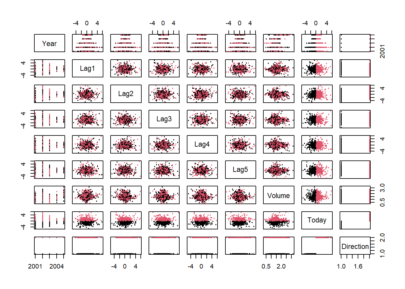
# Create a dataframe for data browsing
sm=Smarket

# Bivariate Plot of inter-lag correlations
pairs(Smarket,col=Smarket$Direction,cex=.5, pch=20)

# Logistic regression
glm.fit=glm(Direction~Lag1+Lag2+Lag3+Lag4+Lag5+Volume,
            data=Smarket,family=binomial)
summary(glm.fit)


Call:
glm(formula = Direction ~ Lag1 + Lag2 + Lag3 + Lag4 + Lag5 + 
    Volume, family = binomial, data = Smarket)

Deviance Residuals: 
   Min      1Q  Median      3Q     Max  
-1.446  -1.203   1.065   1.145   1.326  

Coefficients:
             Estimate Std. Error z value Pr(>|z|)
(Intercept) -0.126000   0.240736  -0.523    0.601
Lag1        -0.073074   0.050167  -1.457    0.145
Lag2        -0.042301   0.050086  -0.845    0.398
Lag3         0.011085   0.049939   0.222    0.824
Lag4         0.009359   0.049974   0.187    0.851
Lag5         0.010313   0.049511   0.208    0.835
Volume       0.135441   0.158360   0.855    0.392

(Dispersion parameter for binomial family taken to be 1)

    Null deviance: 1731.2  on 1249  degrees of freedom
Residual deviance: 1727.6  on 1243  degrees of freedom
AIC: 1741.6

Number of Fisher Scoring iterations: 3

glm.probs=predict(glm.fit,type="response") 
glm.probs[1:5]

        1         2         3         4         5 
0.5070841 0.4814679 0.4811388 0.5152224 0.5107812

glm.pred=ifelse(glm.probs>0.5,"Up","Down")
attach(Smarket)
table(glm.pred,Direction)

        Direction
glm.pred Down  Up
    Down  145 141
    Up    457 507

mean(glm.pred==Direction)

[1] 0.5216

# Make training and test set for prediction
train = Year<2005
glm.fit=glm(Direction~Lag1+Lag2+Lag3+Lag4+Lag5+Volume,
            data=Smarket,family=binomial, subset=train)
glm.probs=predict(glm.fit,newdata=Smarket[!train,],type="response") 
glm.pred=ifelse(glm.probs >0.5,"Up","Down")
Direction.2005=Smarket$Direction[!train]
table(glm.pred,Direction.2005)

        Direction.2005
glm.pred Down Up
    Down   77 97
    Up     34 44

mean(glm.pred==Direction.2005)

[1] 0.4801587

#Fit smaller model
glm.fit=glm(Direction~Lag1+Lag2,
            data=Smarket,family=binomial, subset=train)
glm.probs=predict(glm.fit,newdata=Smarket[!train,],type="response") 
glm.pred=ifelse(glm.probs >0.5,"Up","Down")
table(glm.pred,Direction.2005)

        Direction.2005
glm.pred Down  Up
    Down   35  35
    Up     76 106

mean(glm.pred==Direction.2005)

[1] 0.5595238

# Check accuracy rate
106/(76+106)

[1] 0.5824176

# Can you interpret the results?

Assignment Questions

a. What is/are the requirement(s) of LDA?

Linear Discriminant Analysis is a classification system. Though it is sometimes referred to as LDA regression, like Logistic “regression” it is less of a regression modeling and more of a system of classification. The requirements are of LDA are to use it on non-quantitative outcome variables. OLS expects linear continuous relationships, but something in between categories is not a reality. The example in the ISLR Chapter 4 illustrates this well when the outcomes are seizure, stroke, and drug overdose. Here regression cannot understand different categories that are not order or binary.

b. How LDA is different from Logistic Regression?

LDA models the distribution of predictors separately for each of the category classes, rather than considering them as a conditional distribution as is done with logistic regression. It also requires an additional step once this is done which relies on Bayes’ theorem to fliip them into estimates. Logistic regression and LDA can produce very similar results if the distribution of the dependent variable fits normality assumptions. This is of course not always the case though, so LDA is useful when the separation between classes is believed to be large, if X distribution is assumed to be normal but the sample is small, and if there are more than two response classes for a categorical variable.

c. What is ROC?

ROC is a curve visualization that graphs two types of errors: the sensitivity and specificity (positive and false positive rate, respectively). We interpret a ROC but examining the area underneath the curve. The closer to 1, the better we consider the model. We can use these to compare models (i.e. logistic vs. LDA) to determine which is better.

d. What is sensitivity and specificity? Which is more important in your opinion?

Sensitivity over specificity, due to the importance of accurately diagnosing ill people rather than inaccurately diagnosing healthy people.

e. From the following chart, for the purpose of prediction, which is more critical?

If the above considers diagnostics testing as it does in the ISLR text, then I would say that predicting the true positive rate is the most important. This is the outcome with the most impact on humans and false negatives can be caught with other follow up diagnostics. Therefore, sensitivity over specificity is most important.

f. Calculate the prediction error from the following:

Error calculation: total number of incorrect predictions over total number of predictions.

(23+252)/10,000 = 0.0275

This is pretty good, considering the error rate ranges from 0 to 1.